Introduction
This vignette shows how to assign user-defined syllable
identity labels (e.g. a, b,
c, …) to the clusters discovered during segmentation.
Prerequisites: Before reading this vignette, we recommend completing:
- Constructing a SAP Object — SAP object creation
- Longitudinal Bout Detection — Detecting song bouts across development
- Longitudinal Syllable Segmentation — Segmenting song into syllables across development
What you will learn:
- How to inspect raw segment clusters and verify the final syllable inventory in heatmaps
- How to run automatic syllable labelling with
auto_label() - How to refine or override automatic labels with
manual_label()
Overview
Because defining a syllable repertoire is an inherently subjective task relying on a researcher’s specific criteria or project context, we avoid assuming that automated clusters are perfectly accurate out of the box. Syllable labelling bridges the gap between raw, objective data clustering and your final, supervised categorisation.
-
Automatic labelling (
auto_label()) provides a fast and objective initial pass. It uses density-based clustering (DBSCAN) across both temporal position and acoustic features (UMAP) to group similar segments together. -
Manual labelling (
manual_label()) allows you to exercise your expert judgment: reviewing the automated clusters, merging them where appropriate, and assigning standard alphabetic names (e.g., ‘a’, ‘b’, ‘c’) based on your own visual inspection and interpretation.
Combining both approaches ensures accuracy while saving time on large longitudinal datasets.
Load the SAP object
This tutorial continues directly from Longitudinal Syllable Segmentation. Load the SAP object saved at the end of that tutorial:
sap <- readRDS("longitudinal_syllable_analysis.rds")Inspect raw segment clusters
Before assigning letter labels it is useful to view how segments are
distributed across clusters. plot_clusters() renders a
heatmap-style raster where each row is a segment and columns represent
time within the motif, coloured by cluster identity.
plot_clusters(sap, data_type = "segment", ordered = TRUE)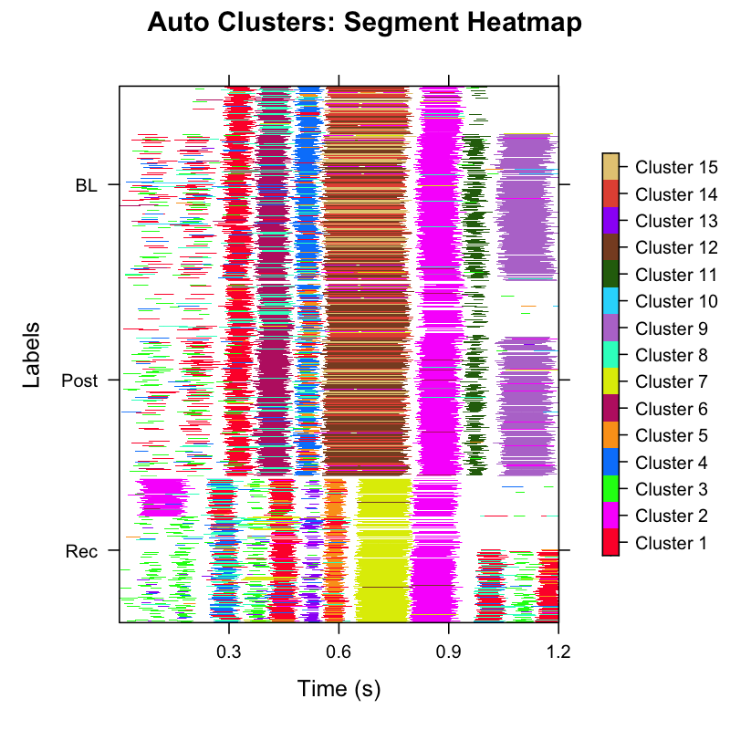
Inspect the output:
- Tight horizontal bands of the same colour → a well-defined syllable type repeats reliably at a fixed position within the motif.
-
Fragmented colours at the same time position → the
cluster boundaries may be too fine; consider re-running
find_clusters()with a lower resolution. - Columns entirely absent → that time position is not consistently detected; check segmentation parameters.
Automatic syllable labelling
auto_label() performs two-stage DBSCAN clustering —
first in temporal space (position and duration within the motif), then
in UMAP acoustic space — to group segments into candidate syllables
automatically.
Key parameters
| Parameter | Role | Default |
|---|---|---|
eps_time |
Temporal separation sensitivity (smaller → more splits) | 0.1 |
eps_umap |
Acoustic similarity sensitivity (smaller → more splits) | 0.6 |
min_pts |
Minimum points to form a cluster | 5 |
weight_time |
Relative weight of time position vs. duration | 4 |
outlier_threshold |
Fraction of total points below which a cluster is discarded | 0.01 |
umap_threshold |
UMAP distance below which two clusters are merged | 1.0 |
sap <- sap |>
  auto_label(
    eps_time          = 0.1,
    eps_umap          = 0.6,
    min_pts           = 5,
    weight_time       = 4,
    outlier_threshold = 0.01,
    umap_threshold    = 1.0
  )
The result is stored in
sap$features$syllable$feat.embeds, which contains a
cluster column with integer cluster IDs. Visualise the
auto-labelled clusters:
sap <- sap |>
  plot_clusters(data_type = "syllable", ordered = TRUE)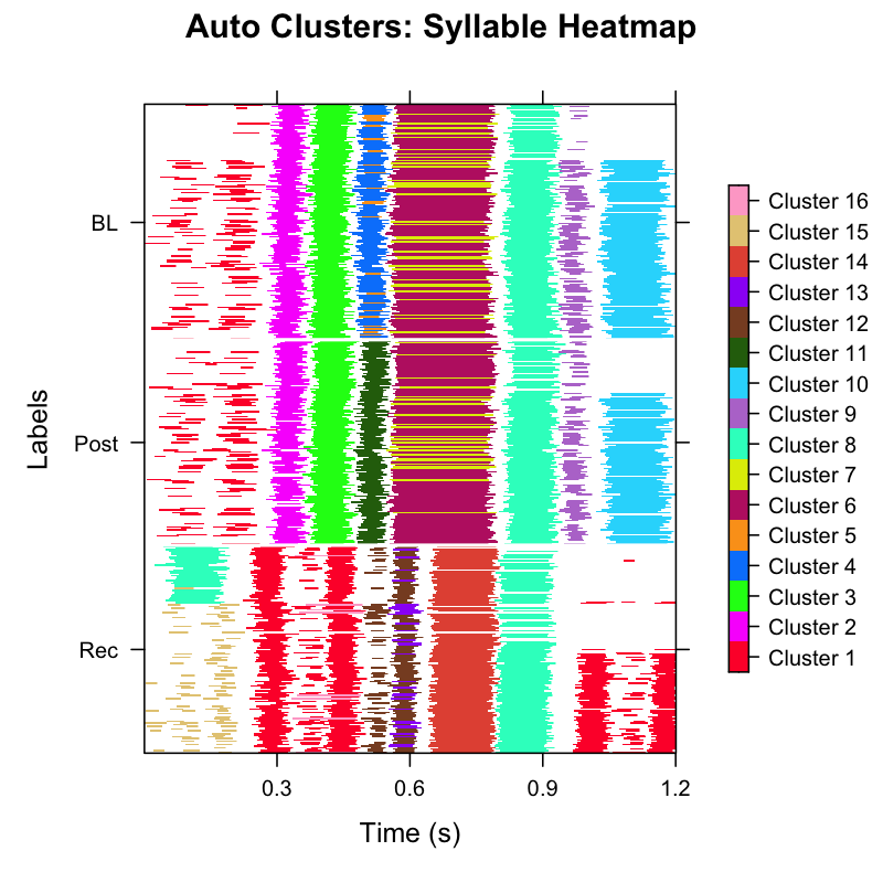
Manual syllable labelling
After auto_label() you know how many integer-coded
clusters exist. Use manual_label() to convert those
integers to the letter codes that match your syllable vocabulary.
Option A — Interactive mode
Run in an interactive R session (e.g. RStudio console) to be prompted for each cluster:
sap <- manual_label(sap, data_type = "syllable", interactive = TRUE)
#> Found clusters: 1, 2, 3, 4, 5, 6, 7, 8, 9, 10, 11, 12, 13, 14
#>
#> Cluster 1:
#> Enter letter (a-z): i
#> Cluster 2:
#> Enter letter (a-z): i
#> Cluster 3:
#> Enter letter (a-z): a
#> ...
Once you have assigned all letters the mapping is stored inside the SAP object and re-used automatically in subsequent calls.
Option B — Predefined label map (reproducible, recommended)
Build a data.frame mapping cluster IDs to letter labels.
Clusters that share the same letter are treated as the same syllable
type. This approach is fully reproducible without
interactive input.
# Inspect the cluster plot above, then define the mapping
map_df <- data.frame(
  cluster = 1:14,
  syllable = c(
    "i", "i", "a", "b", "c", "c",
    "d", "e", "f", "b", "i", "g", "g", "h"
  )
)

sap <- sap |>
  manual_label(
    data_type = "syllable",
    label_map = map_df,
    interactive = FALSE
)Visualise the final syllable inventory
After labelling, inspect the full syllable heatmap and the UMAP coloured by syllable letter to verify consistency across developmental stages.
Heatmap by syllable type
sap <- sap |>
  plot_clusters(label_type = "manual", ordered = TRUE)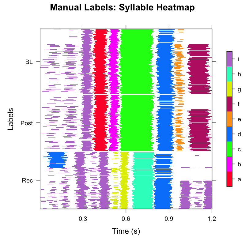
In the manually-labelled heatmap each colour corresponds to one letter-coded syllable. Consistent banding across all three developmental stages (BL, Post, Rec) indicates stable syllable identity.
Accessing syllable data downstream
All labelled syllables are stored in sap$syllables:
head(sap$syllables)
#> filename          day_post_hatch label cluster syllable UMAP1   UMAP2
#> S237_42674.wav    190            BL    4       b        -1.23   2.45
#> S237_42674.wav    190            BL    4       b        -1.01   2.38
#> ...
# Count syllables per type per developmental stage
table(sap$syllables$label, sap$syllables$syllable)| Stage | a | b | c | d | e | f | g | h | i |
|---|---|---|---|---|---|---|---|---|---|
| BL | 156 | 156 | 156 | 148 | 100 | 113 | 0 | 0 | 269 |
| Post | 180 | 180 | 180 | 169 | 118 | 126 | 0 | 0 | 313 |
| Rec | 0 | 0 | 0 | 206 | 0 | 0 | 257 | 171 | 746 |
This table summarizes the total counts of each syllable type across
the three experimental stages. It clearly illustrates how the bird’s
vocal repertoire shifts over time. For example, syllables
a, b, c, e, and
f are sung during the BL (Baseline) and
Post phases, but disappear by the Rec
(Recovery) stage. Conversely, new syllables g and
h emerge exclusively during the Rec stage.
Other syllables, such as d and i, persist
consistently throughout the entire longitudinal period.
Complete labelling pipeline (copy-paste reference)
library(ASAP)

# -- Assumes segmentation pipeline has already been run --
# -- (see Longitudinal Syllable Segmentation vignette)  --

map_df <- data.frame(
  cluster = 1:14,
  syllable = c(
    "i", "i", "a", "b", "c", "c",
    "d", "e", "f", "b", "i", "g", "g", "h"
  )
)

sap <- sap |>
  plot_clusters(data_type = "segment", ordered = TRUE) |> # inspect raw segments
  auto_label() |> # automatic clustering
  plot_clusters(data_type = "syllable", ordered = TRUE) |> # inspect auto clusters # nolint: line_length_linter.
  manual_label(
    data_type = "syllable",
    label_map = map_df,
    interactive = FALSE
  ) |> # assign letter labels
  plot_clusters(label_type = "manual", ordered = TRUE) # final verification
Session info
sessionInfo()
#> R version 4.5.3 (2026-03-11)
#> Platform: x86_64-pc-linux-gnu
#> Running under: Ubuntu 24.04.4 LTS
#>
#> Matrix products: default
#> BLAS:   /usr/lib/x86_64-linux-gnu/openblas-pthread/libblas.so.3
#> LAPACK: /usr/lib/x86_64-linux-gnu/openblas-pthread/libopenblasp-r0.3.26.so;  LAPACK version 3.12.0
#>
#> locale:
#>  [1] LC_CTYPE=C.UTF-8       LC_NUMERIC=C           LC_TIME=C.UTF-8
#>  [4] LC_COLLATE=C.UTF-8     LC_MONETARY=C.UTF-8    LC_MESSAGES=C.UTF-8
#>  [7] LC_PAPER=C.UTF-8       LC_NAME=C              LC_ADDRESS=C
#> [10] LC_TELEPHONE=C         LC_MEASUREMENT=C.UTF-8 LC_IDENTIFICATION=C
#>
#> time zone: UTC
#> tzcode source: system (glibc)
#>
#> attached base packages:
#> [1] stats     graphics  grDevices utils     datasets  methods   base
#>
#> loaded via a namespace (and not attached):
#>  [1] digest_0.6.39     desc_1.4.3        R6_2.6.1          fastmap_1.2.0
#>  [5] xfun_0.57         cachem_1.1.0      knitr_1.51        htmltools_0.5.9
#>  [9] rmarkdown_2.31    lifecycle_1.0.5   cli_3.6.5         sass_0.4.10
#> [13] pkgdown_2.2.0     textshaping_1.0.5 jquerylib_0.1.4   systemfonts_1.3.2
#> [17] compiler_4.5.3    tools_4.5.3       ragg_1.5.2        evaluate_1.0.5
#> [21] bslib_0.10.0      yaml_2.3.12       jsonlite_2.0.0    rlang_1.1.7
#> [25] fs_2.0.1