Constructing SAP Object • ASAP

Introduction

This vignette demonstrates how to construct and organize a SAP (Song Analysis Pipeline) object for longitudinal analysis of zebra finch vocalizations. SAP objects serve as the central data structure in ASAP, managing recordings across multiple developmental time points.

Prerequisites: Before reading this vignette, we recommend completing:

Overview: Basic Audio Analysis - Core ASAP functions
Motif Detection - Template optimization workflow

Compatibility with SAP2011

ASAP is designed to seamlessly work with audio recordings generated by Sound Analysis Pro 2011 (SAP2011), the widely-used software for zebra finch song recording and analysis. The create_sap_object() function automatically extracts metadata from SAP2011’s standardized filename format.

Expected WAV Filename Format

SAP2011 generates WAV files with a specific naming convention that encodes recording metadata:

{bird_id}_{timestamp}_{month}_{day}_{hour}_{minute}_{second}.wav

Example filename:

S237_42674.66837050_10_31_18_33_57.wav
│     │              │  │  │  │  └── Second (57)
│     │              │  │  │  └───── Minute (33)
│     │              │  │  └──────── Hour (18)
│     │              │  └─────────── Day (31)
│     │              └────────────── Month (10 = October)
│     └───────────────────────────── Timestamp (SAP internal)
└─────────────────────────────────── Bird ID (S237)

Extracted Metadata

When you create a SAP object, ASAP automatically parses filenames to extract:

Field	Source	Example
`bird_id`	Filename prefix	“S237”
`day_post_hatch`	Subfolder name	“190”
`recording_date`	Parsed from filename	“10-31”
`recording_time`	Parsed from filename	“18:33:57”
`label`	User-provided	“Baseline”

Organizing Your Recording Data

ASAP expects recordings to be organized in a specific folder structure, where each subfolder represents a developmental time point:

base_path/
├── 190/                  # Day 190 post-hatch
│   ├── S237_42674.66837050_10_31_18_33_57.wav
│   ├── S237_42674.67577440_10_31_18_46_17.wav
│   └── ...
├── 201/                  # Day 201 post-hatch  
│   ├── S237_42685.1754581_11_11_0_29_14.wav
│   └── ...
└── 203/                  # Day 203 post-hatch
    ├── S237_42687.72024667_11_13_20_0_24.wav
    └── ...

Note: Subfolder names are used as day_post_hatch values. While typically numeric days, any consistent naming convention works (e.g., “pre”, “post”, “recovery”).

Creating a SAP Object

library(ASAP)

# Create SAP object from organized recording folders
sap <- create_sap_object(
  base_path = "/path/to/recordings",
  subfolders_to_include = c("190", "201", "203"),
  labels = c("Baseline", "Post", "Recovery")
)

# View the structure
print(sap)
summary(sap)

Example output:

SAP Object
===========
Base path: /path/to/recordings
Time points: 3 (190, 201, 203)
Labels: Baseline, Post, Recovery
Total files: 1247
  - 190 (Baseline): 89 files
  - 201 (Post): 704 files
  - 203 (Recovery): 454 files

Key Arguments

Argument	Description
`base_path`	Root directory containing recording folders
`subfolders_to_include`	Vector of folder names to process (default: all folders)
`subfolders_to_exclude`	Folders to ignore (default: “templates”, “plots”)
`labels`	Human-readable labels for each time point

Exploring SAP Object Contents

# View metadata extracted from filenames
head(sap$metadata)

# Check number of files per time point
table(sap$metadata$label)

# View unique bird IDs
unique(sap$metadata$bird_id)

# Visualize sample recordings
visualize_song(sap, n_samples = 4, random = TRUE)

Example metadata structure:

filename	bird_id	day_post_hatch	recording_date	recording_time	label
S237_42674…wav	S237	190	10-31	18:33:57	Baseline
S237_42685…wav	S237	201	11-11	00:29:14	Post
S237_42687…wav	S237	203	11-13	20:00:24	Recovery

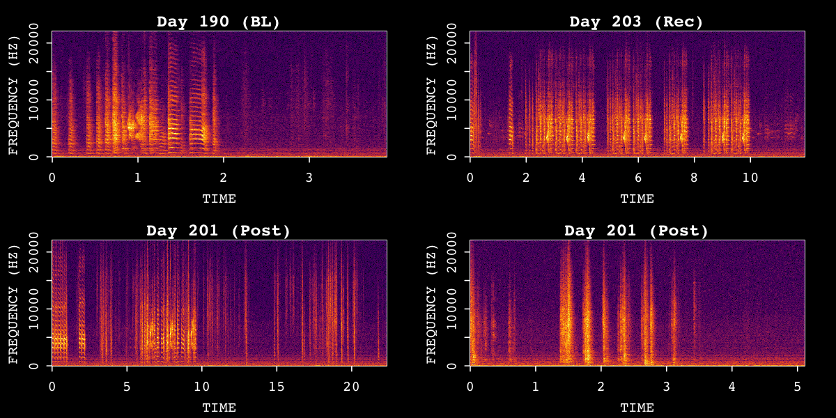
Sample spectrograms from SAP object across time points.

SAP Object Structure

A SAP object contains the following components:

Component	Description
`$base_path`	Root directory path
`$metadata`	Data frame with file information (extracted from filenames)
`$templates`	Template storage (after `create_template()`)
`$motifs`	Detected motifs (after `find_motif()`)
`$bouts`	Detected bouts (after `find_bout()`)
`$features`	Extracted features (after `analyze_spectral()`)

Working with Non-SAP2011 Recordings

ASAP was designed with flexibility in mind. If your recordings are not from SAP2011, you have several options:

Option 1: Create a Wrapper Function

You can write a simple wrapper function to rename your files to match the SAP2011 naming convention. This allows you to use all SAP object functionality directly:

# Example: Convert custom filenames to SAP format
rename_to_sap_format <- function(input_dir, output_dir, bird_id) {
  files <- list.files(input_dir, pattern = "\\.wav$", full.names = TRUE)
  
  for (f in files) {
    # Extract timestamp from your custom format
    # Then create SAP-compatible filename
    timestamp <- as.numeric(Sys.time())
    time_parts <- format(Sys.time(), "%m_%d_%H_%M_%S")
    new_name <- sprintf("%s_%.5f_%s.wav", bird_id, timestamp, time_parts)
    
    file.copy(f, file.path(output_dir, new_name))
  }
}

Option 2: Custom Metadata Object

For datasets that don’t follow ASAP’s naming convention—or for multi-modal experiments with synchronized neural/behavioral data—you can create a custom metadata object directly.

# List your audio files
my_files <- list.files("/path/to/recordings", pattern = "\\.wav$", 
                        recursive = TRUE, full.names = TRUE)

# Create metadata with your own parsing logic
my_metadata <- data.frame(
  filename = basename(my_files),
  bird_id = extract_bird_id(my_files),
  day_post_hatch = extract_day(my_files),
  recording_date = extract_date(my_files),
  recording_time = extract_time(my_files),
  label = assign_labels(my_files),
  
  # Optional: add columns for multi-modal synchronization
  photometry_file = get_matched_photometry(my_files),
  neural_timestamp = get_neural_sync(my_files),
  stringsAsFactors = FALSE
)

This approach supports integration with fiber photometry, electrophysiology, or behavioral video data. For a complete example, see: Juvenile DA Analysis - Data Processing

Next Steps

Once you have created a SAP object, proceed to:

Longitudinal Motif Detection - Apply templates matching across all recordings

Session Info

sessionInfo()
#> R version 4.5.2 (2025-10-31)
#> Platform: x86_64-pc-linux-gnu
#> Running under: Ubuntu 24.04.3 LTS
#> 
#> Matrix products: default
#> BLAS:   /usr/lib/x86_64-linux-gnu/openblas-pthread/libblas.so.3 
#> LAPACK: /usr/lib/x86_64-linux-gnu/openblas-pthread/libopenblasp-r0.3.26.so;  LAPACK version 3.12.0
#> 
#> locale:
#>  [1] LC_CTYPE=C.UTF-8       LC_NUMERIC=C           LC_TIME=C.UTF-8       
#>  [4] LC_COLLATE=C.UTF-8     LC_MONETARY=C.UTF-8    LC_MESSAGES=C.UTF-8   
#>  [7] LC_PAPER=C.UTF-8       LC_NAME=C              LC_ADDRESS=C          
#> [10] LC_TELEPHONE=C         LC_MEASUREMENT=C.UTF-8 LC_IDENTIFICATION=C   
#> 
#> time zone: UTC
#> tzcode source: system (glibc)
#> 
#> attached base packages:
#> [1] stats     graphics  grDevices utils     datasets  methods   base     
#> 
#> loaded via a namespace (and not attached):
#>  [1] digest_0.6.39     desc_1.4.3        R6_2.6.1          fastmap_1.2.0    
#>  [5] xfun_0.56         cachem_1.1.0      knitr_1.51        htmltools_0.5.9  
#>  [9] rmarkdown_2.30    lifecycle_1.0.5   cli_3.6.5         sass_0.4.10      
#> [13] pkgdown_2.2.0     textshaping_1.0.5 jquerylib_0.1.4   systemfonts_1.3.2
#> [17] compiler_4.5.2    tools_4.5.2       ragg_1.5.1        evaluate_1.0.5   
#> [21] bslib_0.10.0      yaml_2.3.12       jsonlite_2.0.0    rlang_1.1.7      
#> [25] fs_1.6.7