Longitudinal Bout Detection • ASAP

Introduction

This vignette demonstrates how to detect and analyze song bouts across longitudinal recordings using SAP objects. Bout detection identifies continuous periods of vocalization, which is essential for understanding song production patterns during development.

Prerequisites: Before reading this vignette, we recommend completing:

Overview: Basic Audio Analysis - Core ASAP functions
Constructing SAP Object - SAP object creation
Longitudinal Motif Detection - Motif-based workflow

Overview

What are bouts? Song bouts are continuous periods of vocalization separated by silence. In zebra finches, a bout typically contains multiple motif renditions and provides important context for understanding song structure and production.

Why detect bouts? Bout-level analysis enables:

Tracking song production rate across development
Analyzing bout duration and structure changes
Understanding motif density within bouts
Identifying practice patterns and song maturation

Relationship to motif detection: While motif detection identifies specific, repeatable vocal sequences, bout detection captures the broader temporal structure of vocalization. When used together (with summary = TRUE), you can analyze how motifs are organized within bouts across developmental time points.

Complete Pipeline

The bout detection workflow processes all recordings in a SAP object to identify bouts across multiple time points.

Option 1: Load SAP Object from Previous Analysis

If you’ve already completed motif detection (see Longitudinal Motif Detection), you can load that SAP object and add bout detection:

library(ASAP)

# Load SAP object from previous motif detection vignette
sap <- readRDS("longitudinal_motif_analysis.rds")

# Add bout detection with motif-bout relationships
sap <- sap |>
  find_bout(
    rms_threshold = 0.1,
    min_duration = 0.4,
    gap_duration = 0.3,
    freq_range = c(3, 5),
    summary = TRUE  # Include motif-bout relationships
  )

# Visualize results
plot_heatmap(sap, segment_type = "bouts", balanced = TRUE)

Option 2: Create New SAP Object

Alternatively, you can create a new SAP object from scratch (see Constructing SAP Object for detailed instructions):

library(ASAP)

# Create SAP object
sap <- create_sap_object(
  base_path = "/path/to/recordings",
  subfolders_to_include = c("190", "201", "203"),
  labels = c("BL", "Post", "Rec")
)

# Detect bouts across all recordings
sap <- sap |>
  find_bout(
    rms_threshold = 0.1,
    min_duration = 0.4,
    gap_duration = 0.3,
    freq_range = c(3, 5)
  )

Note: When creating a new SAP object without prior motif detection, summary = TRUE will not add motif-bout relationship columns (n_motifs, align_time, etc.). Additionally, because template matching is not performed, it is possible to detect false positives such as innate vocalizations or background noise.

Understanding SAP Object Behavior

The find_bout() function processes recordings based on the SAP object’s metadata:

Lazy loading: Audio files are read on-demand during processing
Centralized storage: Results are stored in sap$bouts
Optional visualizations: Set save_plot = TRUE to save detection plots
Parallel processing: Uses multiple cores for efficient batch processing

Example Output

# View bout detection summary
summary(sap$bouts)

# Example output:
#   filename        day_post_hatch label selec start_time end_time n_motifs
#   S237_190_1.wav  190           BL    1     2.45       8.32     12
#   S237_190_1.wav  190           BL    2     15.67      19.84    8
#   S237_201_1.wav  201           Post  1     3.21       10.45    15

When summary = TRUE is enabled with existing motif data, additional columns are included:

n_motifs: Number of motifs detected within each bout
align_time: Time of first motif (useful for alignment)
bout_number_day: Sequential bout number within each day
bout_gap: Time interval from previous bout (within same file)

(Optional) Saving SAP Object

After completing bout detection, you can save the SAP object for later use:

# Save the SAP object with bout detection results
saveRDS(sap, "longitudinal_bout_analysis.rds")

# Later, load it back
sap <- readRDS("longitudinal_bout_analysis.rds")

What gets saved: - All metadata and file references - Bout detection results - Motif data (if previously detected) - All spectral features and analysis results

Important notes: - The original WAV files are not included in the saved object - You must keep the WAV files at their original paths to run additional analyses - The saved .rds file is typically much smaller than the audio data

Visualizing Results

Bout Spectrograms

Visualize sample bouts from each time point to verify detection quality:

# Visualize 3 random bouts per time point
visualize_segments(sap, segment_type = "bouts", n_samples = 3, by_column = TRUE)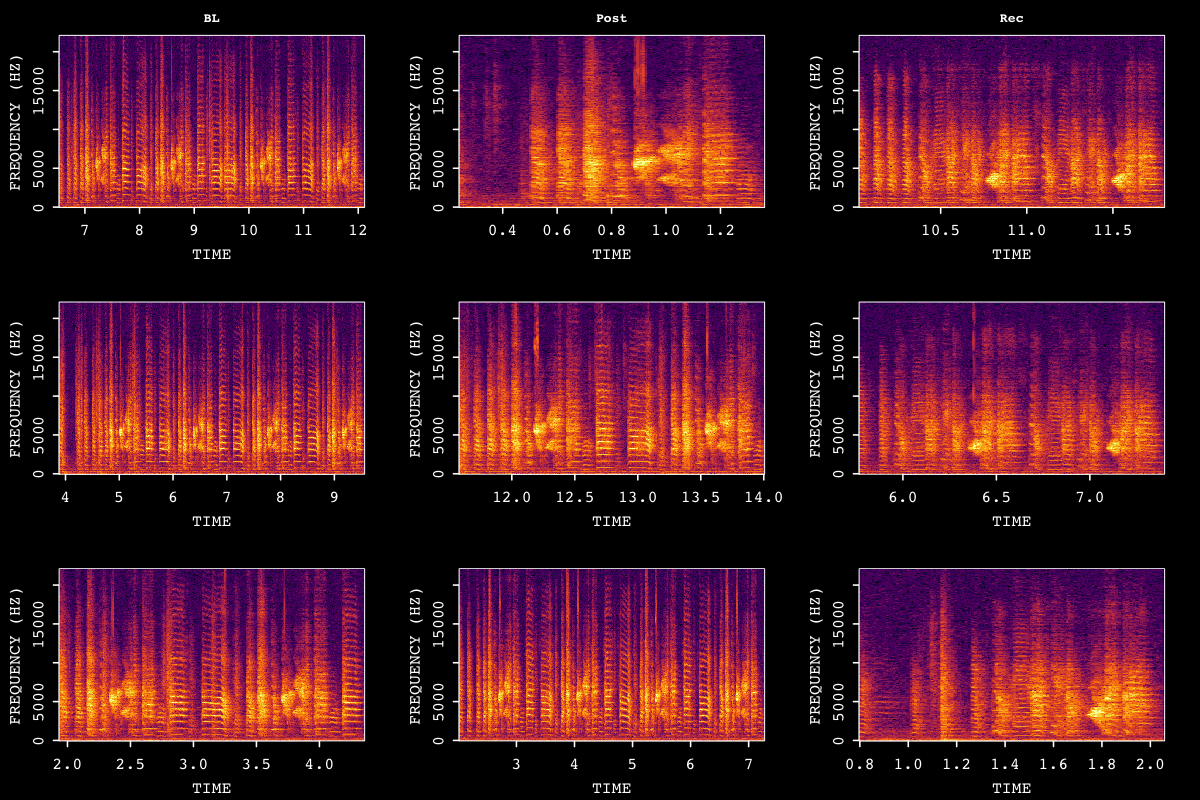

Sample Bouts Across Time Points

Amplitude Envelope Heatmap

Amplitude envelope heatmaps visualize the temporal structure of detected bouts across song developmental stages.

# Create amplitude envelope heatmap with balanced sampling
plot_heatmap(sap, segment_type = "bouts", balanced = TRUE)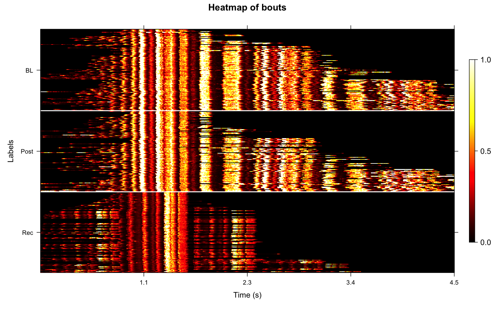

Bout Amplitude Envelope Heatmap

The balanced argument ensures equal representation across time points (e.g., same number of bouts from each developmental stage), which improves statistical comparisons of bout structure across development.

Bout Summary Statistics

Understanding Summary Metrics

When summary = TRUE is enabled and motif data exists, find_bout() calculates additional metrics that reveal the relationship between bouts and motifs.

Example bout summary table (showing first 10 bouts):

Bout Summary Statistics Table

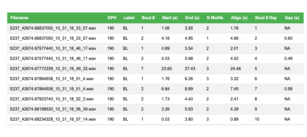
The table includes all detected bouts with the following columns:

n_motifs: Count of motifs within each bout
- Reveals motif density and bout complexity
- Typically increases during song development
align_time: Timestamp of first motif in bout
- Useful for aligning bouts across recordings
- Enables time-locked analysis of bout structure
bout_number_day: Sequential bout number within each day
- Tracks bout order within recording sessions
- Useful for analyzing practice patterns
bout_gap: Time interval from previous bout
- Measures inter-bout intervals
- Reveals temporal patterns in song production

Interpreting Developmental Changes

Bout statistics can reveal important developmental patterns. The plots below show three key bout metrics across developmental stages:

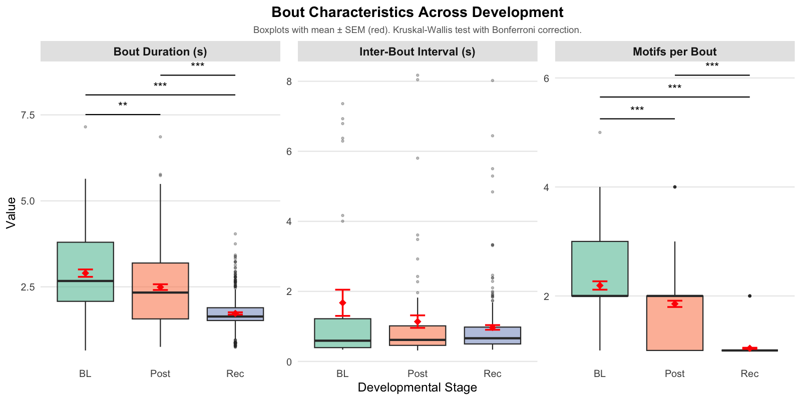
Developmental Trends in Bout Structure

Understanding the visualization:

Boxplots (colored boxes and whiskers):
- Box: Middle 50% of data (interquartile range, IQR)
- Line in box: Median value
- Whiskers: Extend to 1.5× IQR or min/max values
- Small dots: Individual outliers beyond whiskers
Red diamonds with error bars:
- Diamond: Mean (average) value
- Error bars: Standard error of the mean (SEM = SD/√n)
Significance brackets (if present):
- Lines above boxes show significant pairwise differences
- * p < 0.05, ** p < 0.01, *** p < 0.001

Statistical Analysis:

Non-parametric testing is used because temporal birdsong metrics often show skewed distributions and non-constant variance across development:

Kruskal-Wallis Test: An overall test to determine if significant differences exist across the three stages (BL, Post, Rec).
Pairwise Wilcoxon Tests: Post-hoc comparisons to identify specific differences between pairs of stages (e.g., comparing Baseline to Recovery).
Bonferroni Correction: Applied to p-values to adjust for multiple comparisons and prevent false discoveries.
Significance Markers: Brackets and stars (*) in the plot indicate significant pairwise differences based on these adjusted p-values.

Summary of Vocal Bout Changes: - Bouts become progressively shorter and contain fewer motifs from BL to Post to Rec. - The timing between bouts remains unchanged across stages.

Key Parameters for Bout Detection

Understanding and optimizing these parameters is crucial for accurate bout detection:

Parameter	Description	Default	Optimization Tips
`rms_threshold`	Amplitude threshold for bout detection	0.1	Lower = more sensitive (detects quieter bouts) Higher = more selective (only loud bouts) Adjust based on recording quality and background noise
`min_duration`	Minimum bout duration (seconds)	0.5	Filter out brief vocalizations Typical range: 0.4-0.7s Shorter for juvenile birds, longer for adults
`gap_duration`	Minimum silence between bouts (seconds)	0.3	Defines bout boundaries Typical: 0.3s Longer gaps = fewer, longer bouts
`freq_range`	Bandpass filter range (kHz)	c(3, 5)	Focus on vocalization frequencies Zebra finch: c(2, 8) or c(3, 5) Adjust for species-specific frequencies
`edge_window`	Time window for edge effects (seconds)	0.05	Handles recording start artifacts Rarely needs adjustment
`norm_method`	RMS normalization method	“quantile”	“quantile” = robust to outliers “max” = sensitive to peaks
`summary`	Include motif-bout statistics	FALSE	Set TRUE when motif data exists Adds n_motifs, align_time, bout_gap
`balanced`	Balance samples across time points	FALSE	Use TRUE for statistical comparisons Ensures equal representation
`save_plot`	Save detection visualizations	FALSE	Set TRUE to review detection quality Plots saved to base_path/plots/bout_detection/
`plot_percent`	Percentage of files to plot	10	When save_plot = TRUE 10% provides good sampling

Tips for Longitudinal Bout Analysis

1. Optimize Parameters First

Test parameters on representative files from each time point before processing the entire dataset:

# Test on a single file
test_file <- file.path(sap$base_path, "190", sap$metadata$filename[1])

# Try different thresholds
bouts_low <- find_bout(test_file, rms_threshold = 0.05, plot = TRUE)
bouts_med <- find_bout(test_file, rms_threshold = 0.1, plot = TRUE)
bouts_high <- find_bout(test_file, rms_threshold = 0.15, plot = TRUE)

# Compare results
cat("Low threshold:", nrow(bouts_low), "bouts\n")
cat("Medium threshold:", nrow(bouts_med), "bouts\n")
cat("High threshold:", nrow(bouts_high), "bouts\n")

2. Check Detection Quality

Always visualize sample detections to verify bout boundaries are accurate:

# Save plots for manual review
sap <- sap |>
  find_bout(
    min_duration = 0.4,
    save_plot = TRUE,
    plot_percent = 20  # Review 20% of files
  )

# Check plots in: base_path/plots/bout_detection/

3. Use Summary Statistics

Enable summary = TRUE when you have motif data to understand bout-motif relationships:

# Requires existing motif detection
sap <- sap |>
  find_motif(template_name = "d", pre_time = 0.7, lag_time = 0.5) |>
  find_bout(min_duration = 0.4, summary = TRUE)

# Now you can analyze motif density in bouts
sap$bouts |>
  group_by(label) |>
  summarise(avg_motifs_per_bout = mean(n_motifs, na.rm = TRUE))

4. Balance Sampling for Comparisons

Use balanced = TRUE when creating visualizations or statistics for cross-timepoint comparisons:

# Balanced heatmap for fair comparison
sap |> plot_heatmap(segment_type = "bouts", balanced = TRUE)

# Balanced sampling for analysis
balanced_bouts <- select_segments(
  sap$bouts,
  balanced = TRUE
)

5. Consider Recording Quality

Adjust parameters based on recording conditions:

High background noise: Increase rms_threshold, adjust freq_range
Variable amplitude: Use norm_method = "quantile"
Short recordings: Decrease min_duration to capture all bouts
Continuous singing: Increase gap_duration to separate bouts

Session Info

sessionInfo()
#> R version 4.5.2 (2025-10-31)
#> Platform: x86_64-pc-linux-gnu
#> Running under: Ubuntu 24.04.3 LTS
#> 
#> Matrix products: default
#> BLAS:   /usr/lib/x86_64-linux-gnu/openblas-pthread/libblas.so.3 
#> LAPACK: /usr/lib/x86_64-linux-gnu/openblas-pthread/libopenblasp-r0.3.26.so;  LAPACK version 3.12.0
#> 
#> locale:
#>  [1] LC_CTYPE=C.UTF-8       LC_NUMERIC=C           LC_TIME=C.UTF-8       
#>  [4] LC_COLLATE=C.UTF-8     LC_MONETARY=C.UTF-8    LC_MESSAGES=C.UTF-8   
#>  [7] LC_PAPER=C.UTF-8       LC_NAME=C              LC_ADDRESS=C          
#> [10] LC_TELEPHONE=C         LC_MEASUREMENT=C.UTF-8 LC_IDENTIFICATION=C   
#> 
#> time zone: UTC
#> tzcode source: system (glibc)
#> 
#> attached base packages:
#> [1] stats     graphics  grDevices utils     datasets  methods   base     
#> 
#> loaded via a namespace (and not attached):
#>  [1] digest_0.6.39     desc_1.4.3        R6_2.6.1          fastmap_1.2.0    
#>  [5] xfun_0.56         cachem_1.1.0      knitr_1.51        htmltools_0.5.9  
#>  [9] rmarkdown_2.30    lifecycle_1.0.5   cli_3.6.5         sass_0.4.10      
#> [13] pkgdown_2.2.0     textshaping_1.0.5 jquerylib_0.1.4   systemfonts_1.3.2
#> [17] compiler_4.5.2    tools_4.5.2       ragg_1.5.1        evaluate_1.0.5   
#> [21] bslib_0.10.0      yaml_2.3.12       jsonlite_2.0.0    rlang_1.1.7      
#> [25] fs_1.6.7