Longitudinal Motif Detection
Source:vignettes/longitudinal_motif_detection.Rmd
longitudinal_motif_detection.RmdIntroduction
This vignette demonstrates how to detect and analyze song motifs across longitudinal recordings using SAP objects and optimized template parameters.
Prerequisites: Before reading this vignette, we recommend completing:
- Overview: ASAP 101 - Basic ASAP functions
- Motif Detection - Template optimization workflow
- Constructing SAP Object - SAP object creation
Overview
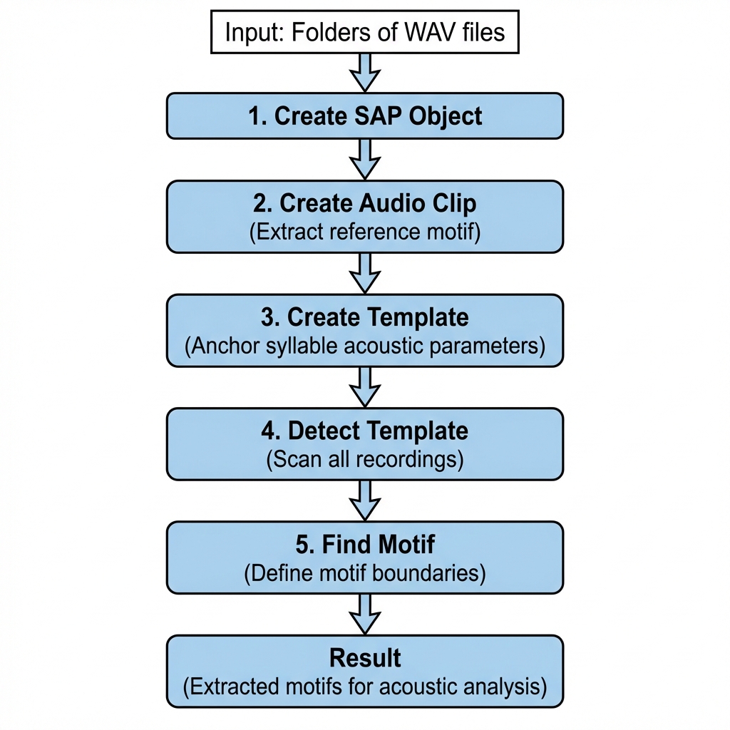
The longitudinal motif detection workflow applies the template parameters you optimized on a single recording (see Motif Detection) across all recordings in a SAP object.
Complete Pipeline
library(ASAP)

# Load or create SAP object
sap <- create_sap_object(
  base_path = "/path/to/recordings",
  subfolders_to_include = c("190", "201", "203"),
  labels = c("BL", "Post", "Rec")
)

# Run the complete motif detection pipeline
sap <- sap |>
  create_audio_clip(
    indices = 1,
    start_time = 1,
    end_time = 2.5,
    clip_names = "motif_ref"
  ) |>
  create_template(
    template_name = "syllable_d",
    clip_name = "motif_ref",
    start_time = 0.72,
    end_time = 0.84,
    freq_min = 1,
    freq_max = 10,
    threshold = 0.5,
    write_template = TRUE
  ) |>
  detect_template(
    template_name = "syllable_d",
    threshold = 0.5,
    proximity_window = 1
  ) |>
  find_motif(
    template_name = "syllable_d",
    pre_time = 0.7,
    lag_time = 0.5
  )
Understanding SAP Object Behavior
1. Metadata-Based Lazy Loading
After creating the SAP object, you have a metadata index (stored in
sap$metadata) that references all audio files by their
paths and timestamps. The actual WAV file data is not loaded
into memory—files are read on-demand during analysis. This
means:
- The SAP object remains lightweight even with thousands of recordings
- All subsequent pipeline steps require the original WAV files to be accessible at their original paths
- If you move or delete the audio files, the pipeline will fail
2. Centralized Result Storage
The SAP object stores all analysis results in a structured format, making it easy to access detection outcomes:
# Access template detection results
sap$templates$template_matches[["syllable_d"]]

# Access extracted motif boundaries (onset/offset timestamps)
sap$motifs  # Data frame with start_time, end_time for each detected motif

# Access spectral features (if analyze_spectral() was run)
sap$features$motif$spectral_feature
3. Optional Template Detection Visualizations
If you set save_plot = TRUE in
detect_template(), spectrogram images of template
detections are saved to a local directory (typically
templates/ within your base path). These images are
not stored in the SAP object but can be useful for
quality control and manual inspection of detection accuracy.
Example output:
=== Starting Template Detection ===

Processing 312 files for day 190 using 7 cores.
Processed files in day 190. Total detections: 1247

Processing 285 files for day 201 using 7 cores.
Processed files in day 201. Total detections: 1089

Processing 250 files for day 203 using 7 cores.
Processed files in day 203. Total detections: 956

Total detections across all days: 3292
Access detection results via: sap$templates$template_matches[["syllable_d"]]
(Optional) Saving SAP Object
After completing the motif detection pipeline, you can save the SAP object for later use or to share with collaborators:
# Save the complete SAP object with all results
saveRDS(sap, "longitudinal_motif_analysis.rds")

# Later, load it back
sap <- readRDS("longitudinal_motif_analysis.rds")
What gets saved: - All metadata and file references - Template detection results - Motif boundaries - Spectral features and UMAP coordinates - Cluster assignments
Important notes: - The original WAV files are
not included in the saved object - You must keep the
WAV files at their original paths to run additional analyses - The saved
.rds file is typically much smaller than the audio data
Visualizing Results
# Visualize sample motifs from each time point
visualize_segments(sap,
  segment_type = "motifs",
  n_samples = 3
)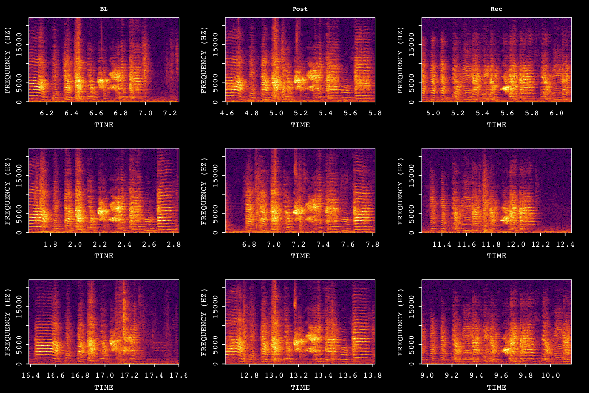
Sample motif spectrograms across developmental time points.
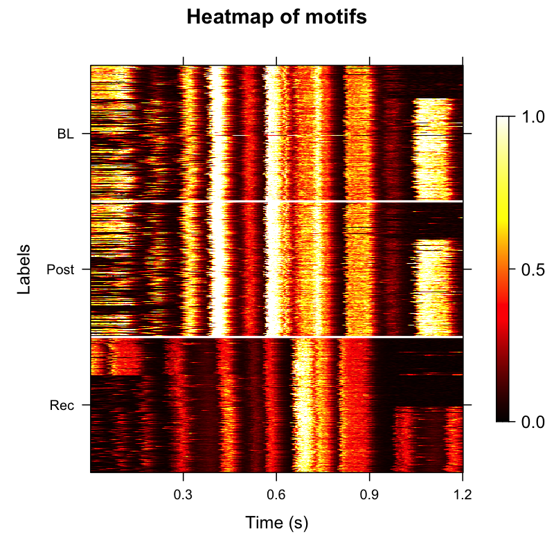
Amplitude Envelope Heatmap
Amplitude envelope heatmaps visualize the temporal structure of
detected motifs. The balanced argument
ensures equal representation across time points (e.g., same number of
motifs from each developmental stage), which improves statistical
comparisons.
However, motif durations can vary across renditions—some motifs may be shorter than others due to natural variability or developmental changes. This duration variability can make heatmaps appear misaligned or noisy, with vertical bands appearing blurred or offset. To address this issue, we can extract acoustic features from individual motifs, cluster them based on these features within each developmental stage, and order them by their latent feature structure (see “Ordered Heatmap” section below).
# Create amplitude envelope heatmap with balanced sampling
plot_heatmap(sap, balanced = TRUE)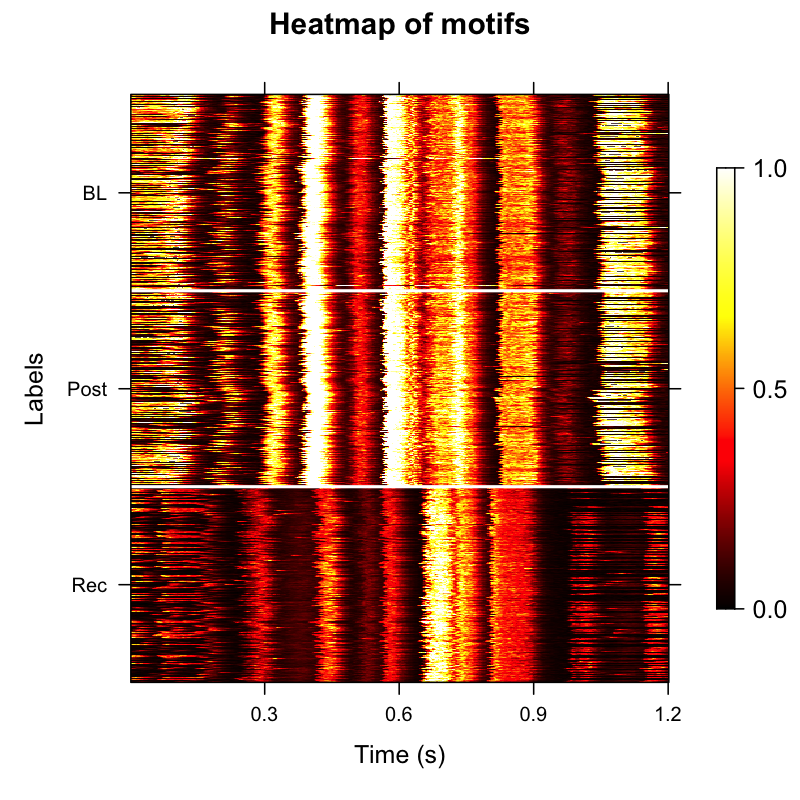
Amplitude envelope heatmap showing temporal structure across time points.
Exporting Motif Clips
Once motifs are detected, you may want to export them as individual
audio files for external analysis, sharing, or manual review. The
create_motif_clips() function makes this easy by extracting
the audio segments for your detected motifs and saving them in an
organized directory structure.
# Export up to 200 motifs per day as individual WAV files
sap <- create_motif_clips(
  sap,
  output_format = "wav",
  output_dir = "exported_motifs",
  n_motifs = 200, # randomly sample up to 200 motifs per day
  amp_normalize = "peak", # Normalize amplitude to prevent clipping
  verbose = TRUE
)
By default, this will organize the exported .wav files
into a clean folder hierarchy
(exported_motifs/motifs/{bird_id}/{day_post_hatch}/motif_xxx.wav)
and automatically generate a companion metadata.csv
containing the timing and source information for each audio clip.
Exporting as HDF5
For large-scale datasets or machine learning workflows, you can export all clips into a single HDF5 file instead of individual WAV files. This keeps everything self-contained and is faster to load in Python or R:
sap <- create_motif_clips(
  sap,
  output_format = "hdf5",
  output_dir    = "exported_motifs",
  n_motifs      = 200,
  hdf5_filename = "motifs.h5"
)
For a full walkthrough of exporting options across different scenarios, see the Exporting Curated Song Clips vignette.
Feature Extraction and Analysis
Extracting spectral features allows you to quantify motif acoustic properties and identify clusters of similar motifs. This is particularly useful for:
- Grouping motifs by acoustic similarity rather than just temporal alignment
- Identifying developmental changes in song structure
- Reducing noise in downstream visualizations
# Extract spectral features (frequency, entropy, duration, etc.)
sap <- sap |>
  analyze_spectral(balanced = TRUE) |>
  find_clusters() |> # Group acoustically similar motifs
  run_umap() # Dimensionality reduction for visualization

# Visualize UMAP by time point
plot_umap(sap, split.by = "label")
Results interpretation:
-
analyze_spectral()extracts ~30 acoustic features per motif (mean frequency, entropy, duration, spectral slope, etc.) and stores them insap$features$motif$spectral_feature -
find_clusters()uses hierarchical clustering to group motifs by acoustic similarity, adding aclustercolumn to the feature data -
run_umap()reduces high-dimensional feature space to 2D for visualization, storing coordinates insap$umap$motif
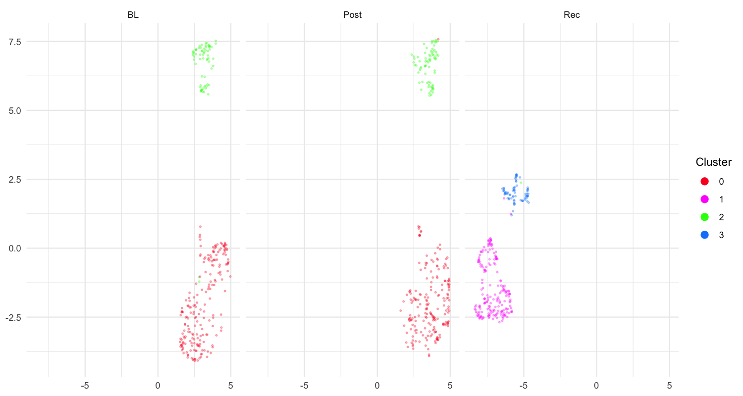
UMAP visualization of motif features colored by developmental time point.
Ordered Heatmap by Acoustic Similarity
After extracting features and clustering, motifs are ordered by their cluster membership and latent feature structure rather than chronological order. Typically, ordering motifs by acoustic similarity creates a cleaner, more organized heatmap that addresses the visual noise from duration variability.
# Create heatmap ordered by cluster membership
plot_heatmap(sap, balanced = TRUE, ordered = TRUE)
Why this helps:
- Motifs with similar acoustic properties are grouped together
- Vertical bands align better because acoustically similar motifs tend to have similar durations
- Developmental patterns become more apparent when organized by acoustic structure
- Reduces visual noise from duration variability
Ordered amplitude envelope heatmap grouped by acoustic similarity.
Key Parameters for Longitudinal Analysis
| Parameter | Location | Description |
|---|---|---|
threshold |
create_template() / detect_template()
|
Minimum correlation score. Adjust in detect_template()
to refine without recreating template. |
proximity_window |
detect_template() |
Filter duplicate detections within this time window (seconds). |
balanced |
analyze_spectral() / plot_heatmap()
|
Balance samples across time points. |
Tips for Longitudinal Analysis
Optimize parameters first: Use the single-file workflow in Motif Detection before bulk processing.
Check detection quality: Visualize sample detections from each time point to verify template works across developmental stages.
Adjust threshold if needed: If detection rates vary significantly across time points, consider adjusting the threshold in
detect_template().Use balanced sampling: When comparing across time points, use
balanced = TRUEto ensure equal representation.
Session Info
sessionInfo()
#> R version 4.5.3 (2026-03-11)
#> Platform: x86_64-pc-linux-gnu
#> Running under: Ubuntu 24.04.4 LTS
#>
#> Matrix products: default
#> BLAS:   /usr/lib/x86_64-linux-gnu/openblas-pthread/libblas.so.3
#> LAPACK: /usr/lib/x86_64-linux-gnu/openblas-pthread/libopenblasp-r0.3.26.so;  LAPACK version 3.12.0
#>
#> locale:
#>  [1] LC_CTYPE=C.UTF-8       LC_NUMERIC=C           LC_TIME=C.UTF-8
#>  [4] LC_COLLATE=C.UTF-8     LC_MONETARY=C.UTF-8    LC_MESSAGES=C.UTF-8
#>  [7] LC_PAPER=C.UTF-8       LC_NAME=C              LC_ADDRESS=C
#> [10] LC_TELEPHONE=C         LC_MEASUREMENT=C.UTF-8 LC_IDENTIFICATION=C
#>
#> time zone: UTC
#> tzcode source: system (glibc)
#>
#> attached base packages:
#> [1] stats     graphics  grDevices utils     datasets  methods   base
#>
#> loaded via a namespace (and not attached):
#>  [1] digest_0.6.39     desc_1.4.3        R6_2.6.1          fastmap_1.2.0
#>  [5] xfun_0.57         cachem_1.1.0      knitr_1.51        htmltools_0.5.9
#>  [9] rmarkdown_2.31    lifecycle_1.0.5   cli_3.6.5         sass_0.4.10
#> [13] pkgdown_2.2.0     textshaping_1.0.5 jquerylib_0.1.4   systemfonts_1.3.2
#> [17] compiler_4.5.3    tools_4.5.3       ragg_1.5.2        evaluate_1.0.5
#> [21] bslib_0.10.0      yaml_2.3.12       jsonlite_2.0.0    rlang_1.1.7
#> [25] fs_2.0.1