Acoustic Feature Analysis

Introduction

This vignette covers three ASAP functions for examining acoustic structure within a single recording: spectral_entropy(), FF(), and amp_env().

spectral_entropy() measures how tonal or noisy a sound is at each point in time by quantifying how evenly power is spread across frequencies. Zebra finch syllables are often highly structured and may show low entropy, especially for harmonic stack syllables or certain calls; in contrast, noisier syllables, broadband calls, or background noise tend to produce higher-entropy traces.
FF() tracks fundamental frequency (perceived pitch) over time. It is the go-to tool for looking at pitch contours within a single syllable or comparing pitch trajectories across many renditions.
amp_env() extracts the amplitude envelope, summarizing how the overall intensity of sound rises and falls across the duration of a segment.

The vignette walks through how to call each function on a simple time window (provide a file path and start/end times), and then shows how the same functions accept a segment data frame produced by segment() — a natural bridge toward population-level analysis with SAP objects.

Prerequisites: Before reading this vignette, we recommend completing:

Overview: ASAP 101 - Basic ASAP functions

What you will learn:

What kinds of data each function accepts
How to measure spectral structure with entropy (Wiener and Shannon)
How to extract pitch contours with the cepstrum method
How to measure amplitude envelopes and reuse segment data frames for feature analysis

Overview: What Data Do These Functions Accept?

All three functions share a common design: they dispatch on the class of their first argument, so you can pass different kinds of input without changing the function name.

`spectral_entropy()` and `FF()`

Input type	What to pass	Key extra argument
Single WAV file	Character path to `.wav` file	`start_time`, `end_time` (seconds)
Segment data frame	Data frame with `filename`, `start_time`, `end_time` columns	`wav_dir` (directory containing the WAV files)
SAP object	A `Sap` object	`segment_type`, sampling/filtering options
Pre-computed matrix	An entropy or F0 matrix returned by a previous call	— (re-plots the stored matrix)

When x is a character path, start_time and end_time default to the full file duration if omitted.

When x is a data frame, it must contain at least filename, start_time, and end_time columns. A single-row data frame behaves identically to the WAV file method. A multi-row data frame triggers parallel processing and returns an aligned matrix.

`amp_env()`

amp_env() always takes a single-row data frame (segment_row) — the row must contain at least start_time and end_time. Provide wav_dir when the WAV file directory is not embedded in the data frame as an attribute.

amp_env(segment_row, wav_dir = NULL, msmooth = NULL,
        amp_normalize = c("none", "peak", "rms"), plot = FALSE)

Setup

library(ASAP)
#> ASAP v0.3.5 loaded.

wav_file <- system.file("extdata", "zf_example.wav", package = "ASAP")
analysis_start <- 1.5
analysis_end <- 2.5

1. Spectral Entropy Analysis

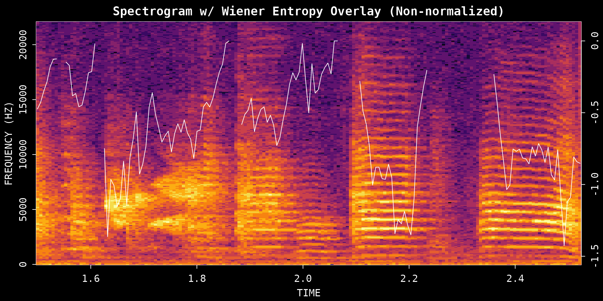
Spectral entropy measures how structured or noisy the frequency distribution is within a sound segment. Harmonic syllables tend to have lower entropy, while broader-band noisy sounds tend to have higher entropy.

Choosing `method` and `normalize`

Two arguments control what the trace looks like:

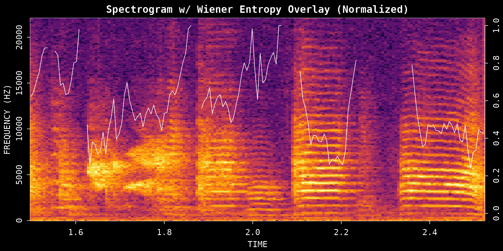
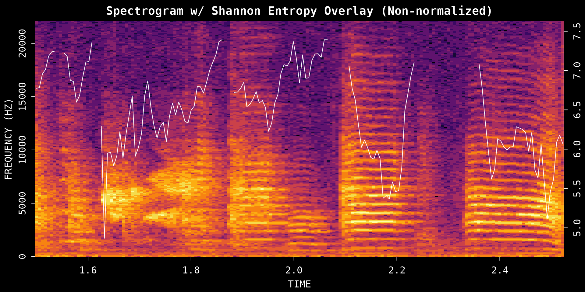
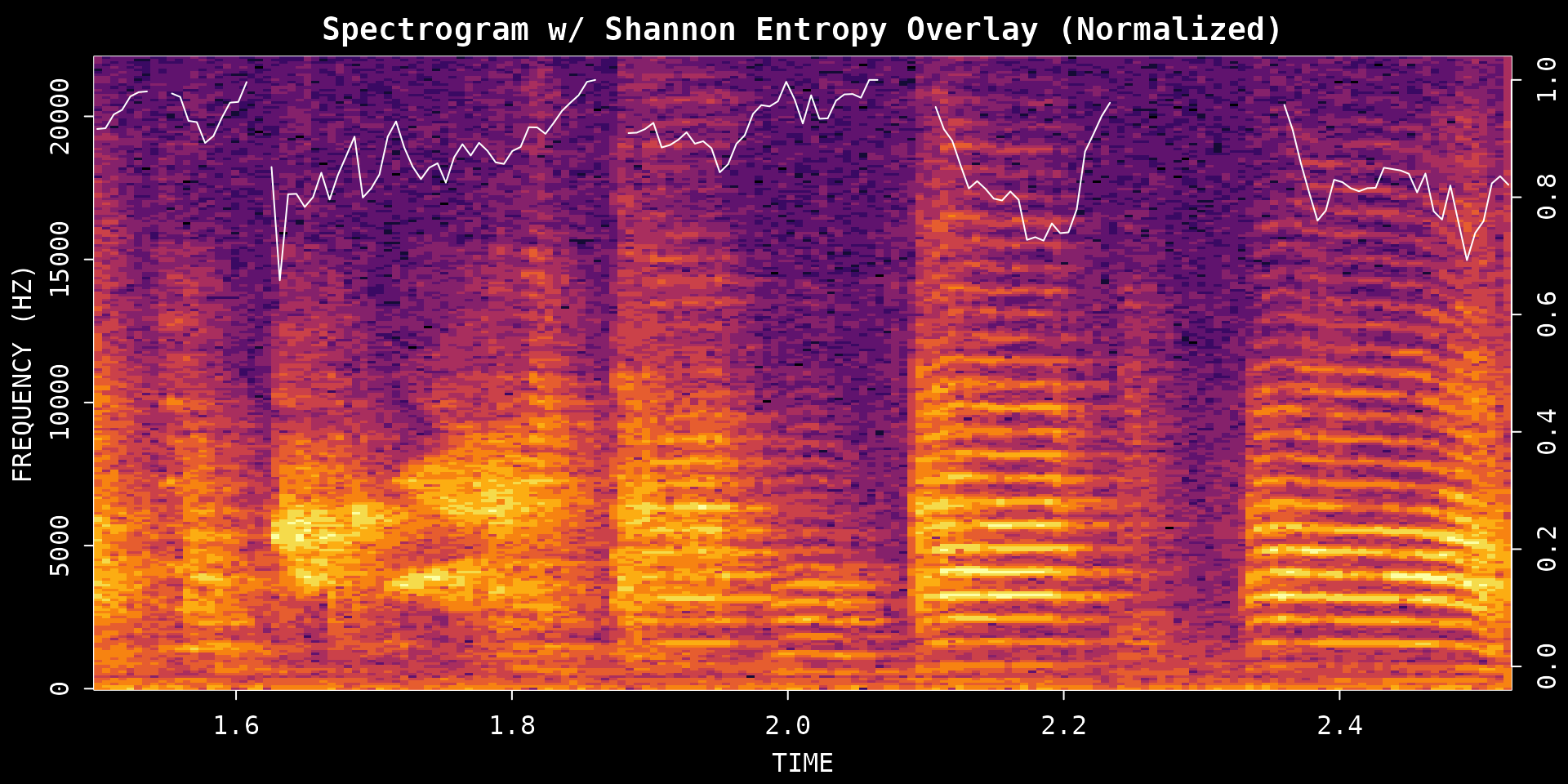
method: "wiener" (default) quantifies spectral flatness — more negative values mean more structured sound, 0 means noise-like. "shannon" quantifies information content — higher values reflect more uniform spectral energy.
normalize: FALSE returns the native scale; TRUE rescales the output to 0–1, making it easier to compare plots across different recordings or methods.

These arguments are independent — you can use either method with or without normalization:

# Wiener entropy, native scale
wiener_raw <- spectral_entropy(
  wav_file,
  start_time = analysis_start,
  end_time   = analysis_end,
  method     = "wiener",
  normalize  = FALSE,
  plot       = TRUE
)

# Wiener entropy, normalized to 0–1
wiener_norm <- spectral_entropy(
  wav_file,
  start_time = analysis_start,
  end_time   = analysis_end,
  method     = "wiener",
  normalize  = TRUE,
  plot       = TRUE
)

# Shannon entropy, native scale
shannon_raw <- spectral_entropy(
  wav_file,
  start_time = analysis_start,
  end_time   = analysis_end,
  method     = "shannon",
  normalize  = FALSE,
  plot       = TRUE
)

# Shannon entropy, normalized to 0–1
shannon_norm <- spectral_entropy(
  wav_file,
  start_time = analysis_start,
  end_time   = analysis_end,
  method     = "shannon",
  normalize  = TRUE,
  plot       = TRUE
)

Argument guide

Argument	Options	How to think about it
`method`	`"wiener"` or `"shannon"`	Use Wiener for spectral flatness (classic bioacoustics metric); use Shannon for information-content style entropy
`normalize`	`FALSE` or `TRUE`	Use `FALSE` to keep the native scale; use `TRUE` for a 0–1 scale that is easier to compare across plots

All four combinations of method × normalize are valid; pick whichever suits your analysis question.

Quality check

Use the plot to compare low-entropy tonal structure against higher-entropy noisy regions. If the segment includes long silent stretches, tighten the time window so the estimate reflects the vocalization itself rather than surrounding silence.

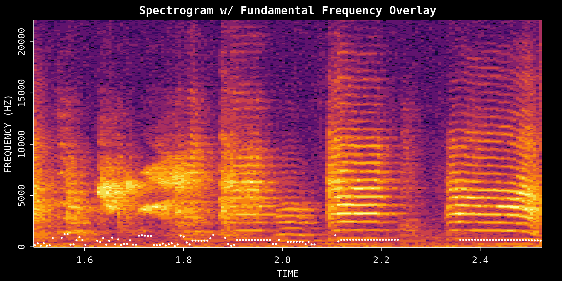
2. Fundamental Frequency (Pitch) Analysis

The FF() function extracts the fundamental frequency contour, showing how perceived pitch changes over time.

The two most important arguments for a single recording are:

method: "cepstrum" or "yin"
fmax: the upper pitch limit to search (Hz)

Cepstrum method

"cepstrum" is the default and the easiest place to start. It is fast and works well for quick inspection of tonal syllables.

pitch_cepstrum <- FF(
  wav_file,
  start_time = analysis_start,
  end_time   = analysis_end,
  method     = "cepstrum",
  fmax       = 1400,
  threshold  = 10,
  plot       = TRUE
)

YIN method

"yin" can be more robust for some signals, but it requires Python dependencies through reticulate, including librosa and numpy.

# ASAP attempts to auto-install librosa/numpy via reticulate when needed.
# This chunk runs only when Python and its dependencies are available;
# it skips gracefully otherwise (e.g. on CRAN or CI build servers).
has_yin <- tryCatch({
  requireNamespace("reticulate", quietly = TRUE) &&
    reticulate::py_module_available("librosa") &&
    reticulate::py_module_available("numpy")
}, error = function(e) FALSE)
#> Downloading uv...Done!

if (has_yin) {
  pitch_yin <- FF(
    wav_file,
    start_time = analysis_start,
    end_time   = analysis_end,
    method     = "yin",
    fmax       = 1400,
    threshold  = 10,
    plot       = TRUE
  )
} else {
  message("YIN method requires Python with librosa and numpy. Skipping.")
}
#> YIN method requires Python with librosa and numpy. Skipping.

Argument guide

Argument	Options	How to think about it
`method`	`"cepstrum"` or `"yin"`	Start with `cepstrum`; try `yin` if you want an alternative pitch tracker and have Python dependencies installed
`fmax`	Numeric upper limit in Hz	Raise it if the contour clips too low; lower it to reduce implausibly high estimates
`threshold`	Confidence filter (%)	Higher values remove uncertain estimates but may introduce gaps

The result contains

f0: Fundamental frequency values over time (kHz)
time: Corresponding time stamps (seconds)

3. Amplitude Envelope from a Syllable Data Frame

The amplitude envelope summarizes how sound intensity changes over time. amp_env() takes a single-row segment data frame with filename, start_time, and end_time columns. A syllable data frame from segment() is a simple way to create that input.

Step 1: Segment a small time window into syllables

syllables <- segment(
  wav_file,
  start_time         = 1,
  end_time           = 5,
  flim               = c(1, 8),
  silence_threshold  = 0.01,
  min_syllable_ms    = 20,
  max_syllable_ms    = 240,
  min_level_db       = 10,
  verbose            = FALSE,
  plot               = FALSE
)

knitr::kable(head(syllables), digits = 3)

filename	selec	threshold	.start	.end	start_time	end_time	duration	silence_gap
zf_example.wav	1	10	0.061	0.123	1.061	1.123	0.061	NA
zf_example.wav	2	10	0.151	0.199	1.151	1.199	0.047	0.028
zf_example.wav	3	10	0.260	0.312	1.260	1.312	0.052	0.061
zf_example.wav	4	10	0.359	0.411	1.359	1.411	0.052	0.047
zf_example.wav	5	10	0.444	0.520	1.444	1.520	0.076	0.033
zf_example.wav	6	10	0.548	0.610	1.548	1.610	0.061	0.028

Step 2: Choose one syllable row

example_syllable <- NULL
if (!is.null(syllables) && nrow(syllables) >= 1) {
  example_syllable <- syllables[1, , drop = FALSE]
  knitr::kable(example_syllable, digits = 3)
}

filename	selec	threshold	.start	.end	start_time	end_time	duration	silence_gap
zf_example.wav	1	10	0.061	0.123	1.061	1.123	0.061	NA

Step 3: Extract the envelope

if (!is.null(example_syllable)) {
  env_syl <- amp_env(
    example_syllable,
    wav_dir       = dirname(wav_file),
    msmooth       = c(256, 50),
    amp_normalize = "peak",
    plot          = TRUE
  )
}

Smoothing and normalization

msmooth: a length-2 vector c(window_samples, overlap_percent). Larger windows smooth out fine-grained amplitude fluctuations; smaller windows preserve rapid transients.
amp_normalize: "none" keeps the raw scale; "peak" scales to the maximum amplitude (good for comparing envelope shapes); "rms" scales by RMS energy (good for comparing absolute loudness).

Argument guide

Argument	Options	How to think about it
`segment_row`	Single-row data frame	Must contain `filename`, `start_time`, `end_time`
`wav_dir`	Path string	Directory containing the WAV files
`msmooth`	Numeric vector c(window, overlap)	Larger window = smoother envelope; smaller = more temporal detail
`amp_normalize`	`"none"`, `"peak"`, `"rms"`	Use `"peak"` when comparing envelope shapes across segments

4. Add-on: Entropy and Pitch from a Segment Data Frame

The same syllable table can also be passed directly to spectral_entropy() and FF(). This is useful when you want to analyze a set of detected segments instead of manually specifying start_time and end_time for each one.

Step 1: Select a few syllable rows

example_syllables <- NULL
if (!is.null(syllables) && nrow(syllables) >= 3) {
  example_syllables <- syllables[1:3, ]
  knitr::kable(example_syllables, digits = 3)
}

filename	selec	threshold	.start	.end	start_time	end_time	duration	silence_gap
zf_example.wav	1	10	0.061	0.123	1.061	1.123	0.061	NA
zf_example.wav	2	10	0.151	0.199	1.151	1.199	0.047	0.028
zf_example.wav	3	10	0.260	0.312	1.260	1.312	0.052	0.061

Step 2: Run spectral entropy on the data frame

The same method and normalize arguments from the single-file examples apply here. Mix and match freely — for example, try method = "shannon" with normalize = FALSE if you prefer the information-content scale.

if (!is.null(example_syllables)) {
  entropy_df <- spectral_entropy(
    example_syllables,
    wav_dir   = dirname(wav_file),
    method    = "wiener",
    normalize = TRUE,
    plot      = TRUE
  )
}

Step 3: Run pitch analysis on the data frame

For data-frame input, FF() aligns the selected segments onto a common time axis and returns a multi-segment result. The method, fmax, and threshold arguments work the same way as for a single WAV file.

if (!is.null(example_syllables)) {
  pitch_df <- FF(
    example_syllables,
    wav_dir   = dirname(wav_file),
    method    = "cepstrum",
    fmax      = 1400,
    threshold = 10,
    plot      = TRUE
  )
}

Summary

These three functions provide a compact toolkit for exploring acoustic variation in a single recording:

Function	What it captures	Primary input types
`spectral_entropy()`	Spectral structure or noisiness	WAV path, data frame, SAP object, pre-computed matrix
`FF()`	Pitch contour over time	WAV path, data frame, SAP object, pre-computed matrix
`amp_env()`	Amplitude dynamics within a segment	Single-row data frame

For motif-scale acoustic analysis across many recordings, continue to the SAP object workflow starting with Constructing SAP Object.

Session Info

sessionInfo()
#> R version 4.5.3 (2026-03-11)
#> Platform: x86_64-pc-linux-gnu
#> Running under: Ubuntu 24.04.4 LTS
#> 
#> Matrix products: default
#> BLAS:   /usr/lib/x86_64-linux-gnu/openblas-pthread/libblas.so.3 
#> LAPACK: /usr/lib/x86_64-linux-gnu/openblas-pthread/libopenblasp-r0.3.26.so;  LAPACK version 3.12.0
#> 
#> locale:
#>  [1] LC_CTYPE=C.UTF-8       LC_NUMERIC=C           LC_TIME=C.UTF-8       
#>  [4] LC_COLLATE=C.UTF-8     LC_MONETARY=C.UTF-8    LC_MESSAGES=C.UTF-8   
#>  [7] LC_PAPER=C.UTF-8       LC_NAME=C              LC_ADDRESS=C          
#> [10] LC_TELEPHONE=C         LC_MEASUREMENT=C.UTF-8 LC_IDENTIFICATION=C   
#> 
#> time zone: UTC
#> tzcode source: system (glibc)
#> 
#> attached base packages:
#> [1] stats     graphics  grDevices utils     datasets  methods   base     
#> 
#> other attached packages:
#> [1] ASAP_0.3.5
#> 
#> loaded via a namespace (and not attached):
#>  [1] rappdirs_0.3.4     sass_0.4.10        generics_0.1.4     tidyr_1.3.2       
#>  [5] lattice_0.22-9     digest_0.6.39      magrittr_2.0.4     evaluate_1.0.5    
#>  [9] grid_4.5.3         RColorBrewer_1.1-3 fastmap_1.2.0      rprojroot_2.1.1   
#> [13] jsonlite_2.0.0     Matrix_1.7-4       tuneR_1.4.7        purrr_1.2.1       
#> [17] scales_1.4.0       pbapply_1.7-4      textshaping_1.0.5  jquerylib_0.1.4   
#> [21] cli_3.6.5          rlang_1.1.7        pbmcapply_1.5.1    fftw_1.0-9        
#> [25] withr_3.0.2        seewave_2.2.4      cachem_1.1.0       yaml_2.3.12       
#> [29] av_0.9.6           tools_4.5.3        parallel_4.5.3     dplyr_1.2.0       
#> [33] ggplot2_4.0.2      here_1.0.2         reticulate_1.45.0  vctrs_0.7.2       
#> [37] R6_2.6.1           png_0.1-9          lifecycle_1.0.5    fs_2.0.1          
#> [41] MASS_7.3-65        ragg_1.5.2         pkgconfig_2.0.3    desc_1.4.3        
#> [45] pkgdown_2.2.0      pillar_1.11.1      bslib_0.10.0       gtable_0.3.6      
#> [49] glue_1.8.0         Rcpp_1.1.1         systemfonts_1.3.2  xfun_0.57         
#> [53] tibble_3.3.1       tidyselect_1.2.1   knitr_1.51         farver_2.1.2      
#> [57] htmltools_0.5.9    patchwork_1.3.2    rmarkdown_2.31     signal_1.8-1      
#> [61] compiler_4.5.3     S7_0.2.1

Introduction

Overview: What Data Do These Functions Accept?

spectral_entropy() and FF()

amp_env()

Setup

1. Spectral Entropy Analysis

Choosing method and normalize

Argument guide

Quality check

2. Fundamental Frequency (Pitch) Analysis

Cepstrum method

YIN method

Argument guide

The result contains

3. Amplitude Envelope from a Syllable Data Frame

Step 1: Segment a small time window into syllables

Step 2: Choose one syllable row

Step 3: Extract the envelope

Smoothing and normalization

Argument guide

4. Add-on: Entropy and Pitch from a Segment Data Frame

Step 1: Select a few syllable rows

Step 2: Run spectral entropy on the data frame

Step 3: Run pitch analysis on the data frame

Summary

Session Info

`spectral_entropy()` and `FF()`

`amp_env()`

Choosing `method` and `normalize`